Healthy Cereals? A Dad's Pursuit of Healthy Kid's Cereals
WHAT MAKES A CEREAL HEALTHY? A RECOMMENDATION
I am using the USDA, FDA, and other reputable sources to determine the attributes of a healthy cereal. I have listed below the standards I will be using for this project.
HEALTHY GUIDELINES
- Sugar content: .25g of sugar for every 4g of cereal.
- (Reference: https://www.fns.usda.gov/tn/choose-breakfast-cereals-are-lower-sugar)
- Fiber at least 3 grams per serving
- Sodium content:
- Low sodium: 5% or less per serving size
- High sodium: 20% or more per serving size
- (Reference: https://www.fda.gov/food/nutrition-education-resources-materials/sodium-your-diet)
NOTE I do not include fat content because fat can be healthy depending on the type which isn’t stated in the dataset. Also, vitamins are not broken into types in this dataset so it is difficult to use that as an indicator since many cereals add vitamins.
library(tidyverse)
library(caret)
library(factoextra)
library(cluster)
library(fpc)
library(fastDummies)
set.seed(15)

# Changed the column types to better represent the types in the columns.
cereal <- read_csv("Cereals.csv",
                   col_types = c("cffiiiiddiiifddd"))

##       name        mfr       type   calories    protein        fat     sodium
## 0.00000000 0.00000000 0.00000000 0.00000000 0.00000000 0.00000000 0.00000000
##      fiber      carbo     sugars     potass   vitamins      shelf     weight
## 0.00000000 0.01298701 0.01298701 0.02597403 0.00000000 0.00000000 0.00000000
##       cups     rating
## 0.00000000 0.00000000
Carbo, sugars, and potass are the only variables with missing values. Removing the three breakfast kinds of cereal with these missing features is acceptable (rows). Also, I noticed that the data for weight measurement uses both imperial and metric-based measures (cups/lbs/ounces vs. grams). I will convert all of the weight measurements to grams. The conversion that I will use is 201.6g per cup and 453.6g per lbs (source: https://www.metric-conversions.org/weight/ounces-to-grams.htm).
# Converted cups/lbs/ounces to grams.
cereal %>%
  mutate(cups = cups * 201.6,
         weight = weight * 453.6) %>%
  rename(serving_size = cups) -> cereal
Normalizing Dataset
# Normalizing the df.

norm <- preProcess(cereal, method = c("scale", "center"))

cereal_norm <- predict(norm, cereal)

summary(cereal_norm)

##      name           mfr    type      calories          protein
##  Length:77          N: 6   C:74   Min.   :-2.9195   Min.   :-1.4116
##  Class :character   Q: 8   H: 3   1st Qu.:-0.3533   1st Qu.:-0.4982
##  Mode  :character   K:23          Median : 0.1600   Median : 0.4152
##                     R: 8          Mean   : 0.0000   Mean   : 0.0000
##                     G:22          3rd Qu.: 0.1600   3rd Qu.: 0.4152
##                     P: 9          Max.   : 2.7262   Max.   : 3.1554
##                     A: 1
##       fat              sodium            fiber              carbo
##  Min.   :-1.0065   Min.   :-1.9047   Min.   :-0.90290   Min.   :-2.50878
##  1st Qu.:-1.0065   1st Qu.:-0.3540   1st Qu.:-0.48333   1st Qu.:-0.71728
##  Median :-0.0129   Median : 0.2424   Median :-0.06375   Median :-0.07745
##  Mean   : 0.0000   Mean   : 0.0000   Mean   : 0.00000   Mean   : 0.00000
##  3rd Qu.: 0.9807   3rd Qu.: 0.6003   3rd Qu.: 0.35582   3rd Qu.: 0.56237
##  Max.   : 3.9614   Max.   : 1.9124   Max.   : 4.97115   Max.   : 2.09795
##                                                         NA's   :1
##      sugars             potass           vitamins       shelf
##  Min.   :-1.60467   Min.   :-1.1883   Min.   :-1.2643   3:36
##  1st Qu.:-0.91953   1st Qu.:-0.7977   1st Qu.:-0.1453   1:20
##  Median :-0.00601   Median :-0.1231   Median :-0.1453   2:21
##  Mean   : 0.00000   Mean   : 0.0000   Mean   : 0.0000
##  3rd Qu.: 0.90751   3rd Qu.: 0.3030   3rd Qu.:-0.1453
##  Max.   : 1.82103   Max.   : 3.2855   Max.   : 3.2115
##  NA's   :1          NA's   :2
##      weight         serving_size         rating
##  Min.   :-3.5195   Min.   :-2.4538   Min.   :-1.7529
##  1st Qu.:-0.1968   1st Qu.:-0.6490   1st Qu.:-0.6757
##  Median :-0.1968   Median :-0.3053   Median :-0.1613
##  Mean   : 0.0000   Mean   : 0.0000   Mean   : 0.0000
##  3rd Qu.:-0.1968   3rd Qu.: 0.7690   3rd Qu.: 0.5811
##  Max.   : 3.1260   Max.   : 2.9176   Max.   : 3.6334
##
One Hot Encoding Variables
# One Hot Encoding "shelf" variable so I can include it in the euclidean
# measurement for distance between points.

cereal_norm <- dummy_cols(cereal_norm,
                          select_columns = c("shelf"),
                          remove_first_dummy = FALSE,
                          remove_selected_columns = TRUE)
The features are normally-distributed as the means are relatively close to the medians.
# Removing the 3 rows with missing values.

cereal_norm <- cereal_norm[complete.cases(cereal_norm), ]
colMeans(is.na(cereal_norm))

##         name          mfr         type     calories      protein          fat
##            0            0            0            0            0            0
##       sodium        fiber        carbo       sugars       potass     vitamins
##            0            0            0            0            0            0
##       weight serving_size       rating      shelf_3      shelf_1      shelf_2
##            0            0            0            0            0            0

# The only hot cereal was "Maypo" and will remove that since my focus
# is on "cold cereals".

cereal_norm <- cereal_norm[-42, -3]
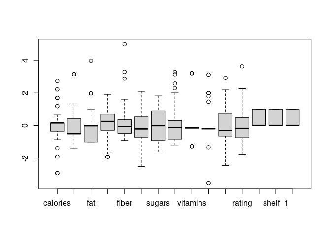
Outliers are Informative in this Dataset
boxplot(cereal_norm[, 3:17])
cereal_norm %>%
  filter(calories> 1 & weight > 0) %>%
  select(name, sugars, shelf_3, rating)

## # A tibble: 6 x 4
##   name                        sugars shelf_3 rating
##   <chr>                        <dbl>   <int>  <dbl>
## 1 Basic_4                    0.222         1 -0.401
## 2 Just_Right_Fruit_&_Nut     0.451         1 -0.441
## 3 Mueslix_Crispy_Blend       1.36          1 -0.879
## 4 Nutri-Grain_Almond-Raisin -0.00601       1 -0.140
## 5 Oatmeal_Raisin_Crisp       0.679         1 -0.870
## 6 Total_Raisin_Bran          1.59          1 -1.00
After investigating the outliers in this dataset, they will be informative for clustering. For example, calories and weight outliers are the same types of cereals. These cereals have lower ratings, higher calories, higher sugar levels, and weight (see above). The higher sugar content is due to the added dried fruits.
Possible Relationships in the Dataset
cor(cereal_norm[, 3:17]) -> cor_cereal
corrplot::corrplot(cor_cereal)
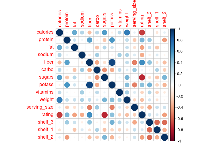
- Positively Correlated
- Fiber and potassium have a high correlation to one another,
- Calorie to weight and sugar,
- Fiber to protein, potassium, fiber, and rating
- Negatively Correlated
- Rating to calories and sugars
Summary
Shelf three has the kinds of cereal that have higher levels of potassium, fiber, and protein.
Shelf two seems to have cereals with higher sugar, low amounts of protein, lower amounts of fiber. These cereals are perfect for kids riding in shopping carts… unless you are the parent…
# Bran based cereals are highest in potassium and also tend to have
# highest amounts of protein.

cereal_norm %>%
  filter(potass > 2 & fiber > 1.5)

## # A tibble: 4 x 17
##   name  mfr   calories protein     fat sodium fiber  carbo sugars potass
##   <chr> <fct>    <dbl>   <dbl>   <dbl>  <dbl> <dbl>  <dbl>  <dbl>  <dbl>
## 1 100%… N       -1.89    1.33  -0.0129 -0.354  3.29 -2.51  -0.234   2.58
## 2 All-… K       -1.89    1.33  -0.0129  1.20   2.87 -2.00  -0.463   3.14
## 3 All-… K       -2.92    1.33  -1.01   -0.235  4.97 -1.74  -1.60    3.29
## 4 Post… P        0.673   0.415 -0.0129  0.481  1.61 -0.973  1.59    2.29
## # … with 7 more variables: vitamins <dbl>, weight <dbl>, serving_size <dbl>,
## #   rating <dbl>, shelf_3 <int>, shelf_1 <int>, shelf_2 <int>
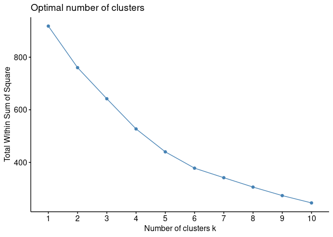
Determining a value for K.
fviz_nbclust(cereal_norm[, 3:17], FUN = hcut, method = "wss")
fviz_nbclust(cereal_norm[, 3:17], FUN = hcut, method = "silhouette")
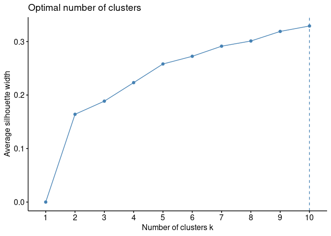
I am going to use the WSS and Silhouette methods to give me a starting point for finding optimal k. Often times there is not a “best” approach to always optimizing k. I will start analyzing k=6 and see how the cereals are grouped and make adjustments if needed from there.
# Set the rownames for the dendrograms.
rownames(cereal_norm) <- cereal_norm$name
# Finding the distance using euclidean method.
d <- get_dist(cereal_norm,
              method = "euclidean")
Why I am using Hierachical Clustering
Hierarchical Clustering
Diversive Analysis Hierarchical Clustering (DIANA) is a clustering algorithm. This algorithm starts with all of our cereals and clusters them into two groups. The algorithm will repeat with the end result being a dendrogram, a family tree but for cereals.
K-Means tends to favor more globular clusters and it only has one method on how the clusters are formed. Hierarchical clusters have many more methods to control how we can link the data to form the clusters. This will be more helpful since I am familiar with the types of cereals in this dataset and inspecting the different methods for clustering in the dendrogram will allow me to choose the best way to cluster the cereals.
Hierarchical Analysis of Cereals
Single Linkage: The Worst Linkage
# Hierarchical clustering using cereal_norm Linkage, Single Linkage,
# Average Linkage, and Ward's Method. Using agnes() to obtain the AC or
# cluster structure strength and using hclust() to plot dendrogram.

# Using "dendextend" to plot more dynamic dendrograms.
library(dendextend)

# creating a dissimilarity matrix based on euclidean distance using
# "complete linkage" method to create the dendrogram.

hc <- hclust(d, method = "single")

# Converting hclust to a dendrogram class so I can visualize it.
dend <- as.dendrogram(hc)

# Setting margins for the graph.
par(mar=c(10,1,1,1))

# Setting labels, branch and label colors, & label size. I repeat the above
# and below steps for the "average linkage", "complete linkage", and "ward
# method" for creating the dendrograms. I will not show the code as the only
# difference is the method is equal to the listed type of linkage.

dend %>%
  set("labels_col",
      value = c("skyblue",
                "firebrick",
                "orange",
                "grey",
                "blue",
                "green"
                ),
      k = 6
      ) %>%
  set("branches_k_color",
      value = c("skyblue",
                "firebrick",
                "orange", "grey",
                "blue",
                "green"
                ),
      k = 6
      ) %>%
  set("nodes_cex", 0.7) %>%
  set("labels_cex", .6) %>%
  plot(axes=FALSE)
# Creating a clustering visualization to see the groupings in 2-dimensions
# for clustering structure comparison.

sub_group <-  cutree(hc, k = 6)
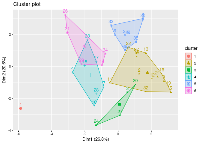
fviz_cluster(list(data = cereal_norm[,3 :17], cluster = sub_group))
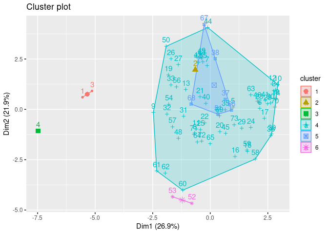
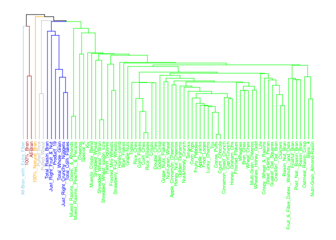
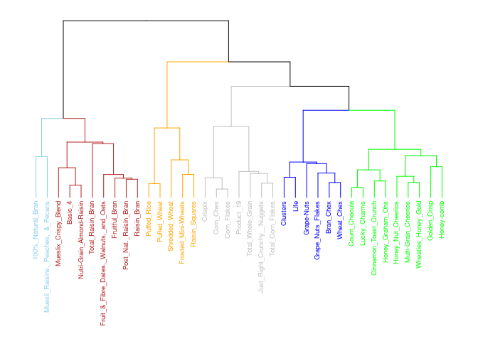
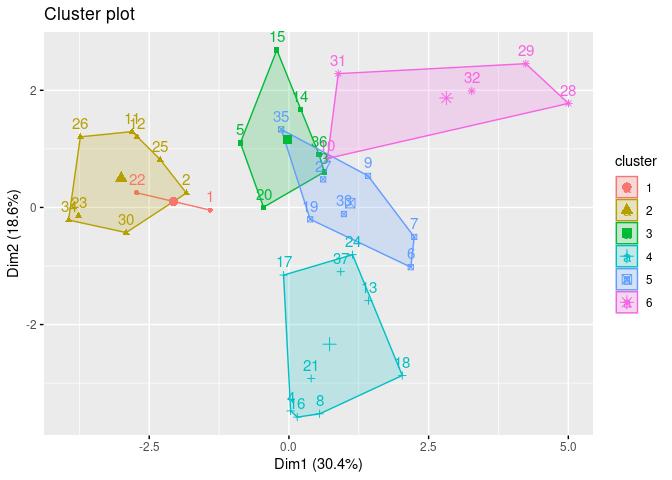
Cluster 2 contains about 85% of all the cereals. The cereals in that cluster are of different types like Trix and Great Grains Pecans. This method did not do a good job clustering the cereals to help me recommend healthy types of cereals.
Average Linkage: Better than Single
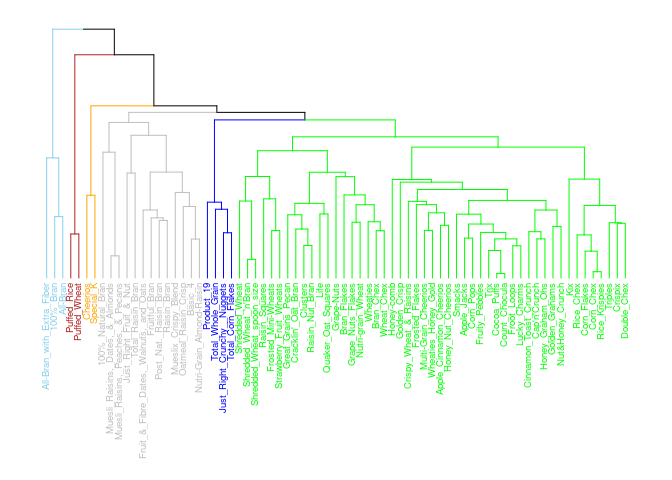
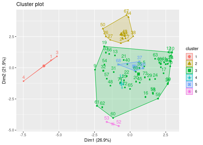
This linkage method looks very similar to single with the exception of the larger cluster having a few small clusters inside of it. It does seem to be an improvement over single linkage as there is more cluster separation and clusters are more compact, comparatively.
Complete Linkage: Second Best Linkage Method
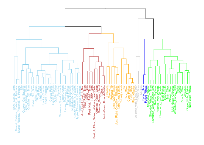
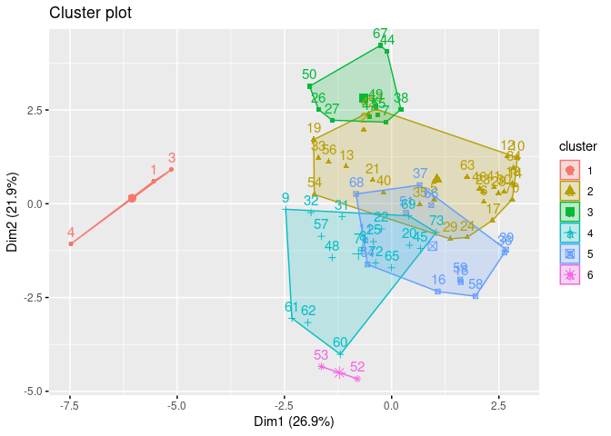
The clusters look fairly separated and fairly uniformly distributed. Cluster 5 overlaps more significantly with 4 and 2. However, looking closer at the dendrogram it does seem that it did a good job grouping the cereals into like categories.
Ward’s Method: The Best Method
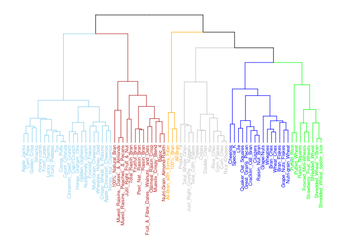
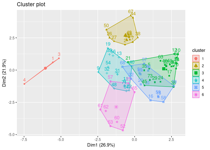
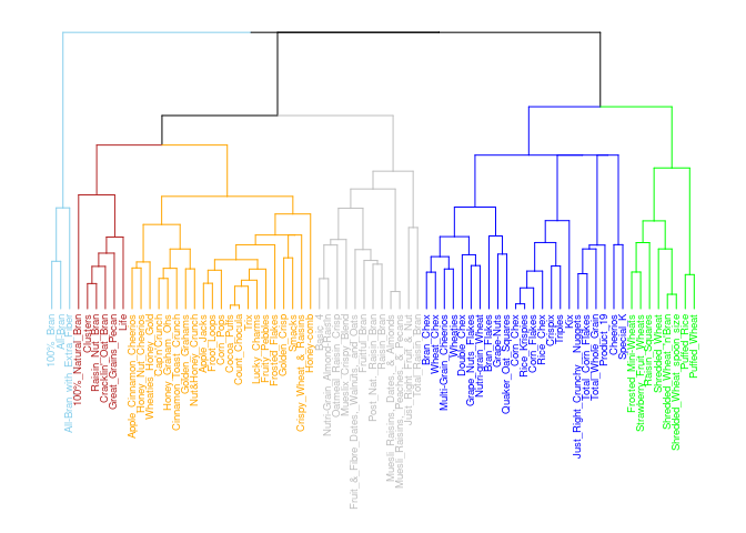
I think Ward’s is the best method for the cereal recommendations as the clusters are more separate and compact (except cluster 3 which overlaps 5). For only having 73 cereals, I think the above dendrogram does a good job of classifying the clusters. For example, All Bran brand cereals are in their own cluster and on the same branch as Grape Nuts, Quaker Oat Squares, etc… While Corn Pops is with Trix and Fruity Pebbles on it’s own branch.
AC Confirms My Analysis
# Agglomerative coefficient with Agnes to determine the strength of
# the cluster structure.
m <- c("average",
       "single",
       "complete",
       "ward"
        )

names(m) <- c("average",
               "single",
               "complete",
               "ward")

# function to compute coefficient
ac <- function(x) {
  agnes(d,
        method = x)$ac
}

map_dbl(m, ac)

##   average    single  complete      ward
## 0.7775099 0.5767978 0.8426844 0.9002626
I am going with the Ward method due to the visualizations and with the strength of the structure being the highest at .90 and due to my analysis aligning with these results as well.
Test Partitioning: Clusters have Very Good Stability
Preparation for Cluster Comparison and Classification
cereal <- cereal[complete.cases(cereal), ] # removing rows with missing values.
cereal <- cereal[-42, -3] # removing Maypo and the Type column.


# attaching the cluster number of each cereal to the normalized dataset.
cereal_norm$cluster <- as.factor(cutree(dend, k = 6))
cereal$cluster <- as.factor(cutree(dend, k = 6))
Creating Partitions
# Split the dataset by 50% randomly using the Caret Package. I choose 50%
# because the dataset is small.

test_split <- createDataPartition(cereal_norm$sugars, p = .5, list = FALSE)
test <- cereal_norm[test_split, ]
row.names(test) <- test$name
Calculating New Distance
#  I am testing to see how well the clustering algorithm will put the
for the test data.

d2 <- get_dist(test,
               method = "euclidean")
Ward’s Method on Test Datset
Cluster Stability Comparison
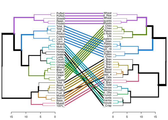
# Looking at the formation of the clusters of the test partition with the original dataset.
# Found the intersection of the orginal dataset with the test partition.

intersect_dend <- intersect_trees(dend1 = dend_test, dend2 = dend)

# Using the dendbackback function in the "dendextend" package to map the two dendrograms back to back.

dendbackback(
  intersect_dend[[1]],
  intersect_dend[[2]],
  sort = TRUE,
  highlight_distinct_edges = FALSE,
  common_subtrees_color_lines = TRUE,
  common_subtrees_color_branches = TRUE)
Very Good Cluster Stability
The dendrogram visualization above shows that only 4 (the black lines) cereals were not grouped in the same cluster with the same cereals. This means that 32 out of the 36 cereals were clustered the same as the original dataset. I would say that is pretty good!
Test Partitioning Trial #2
I am repeating the same process as above so I choose not to show the output since it is simply repeated.
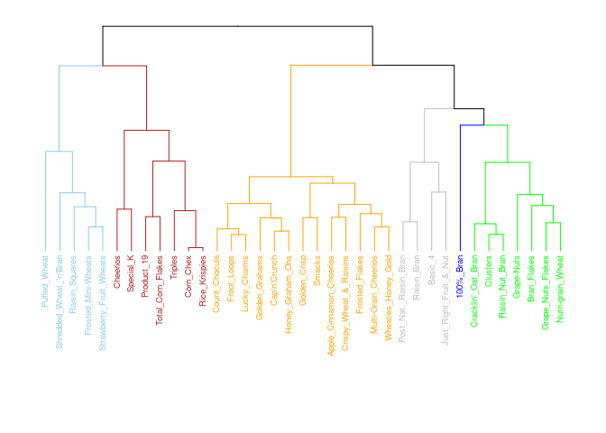
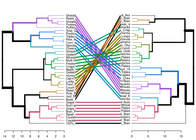
33 (non-black lines) out of the 36 cereals were clustered the same as the original dataset. Again that is really good!
AGNES meets DIANA
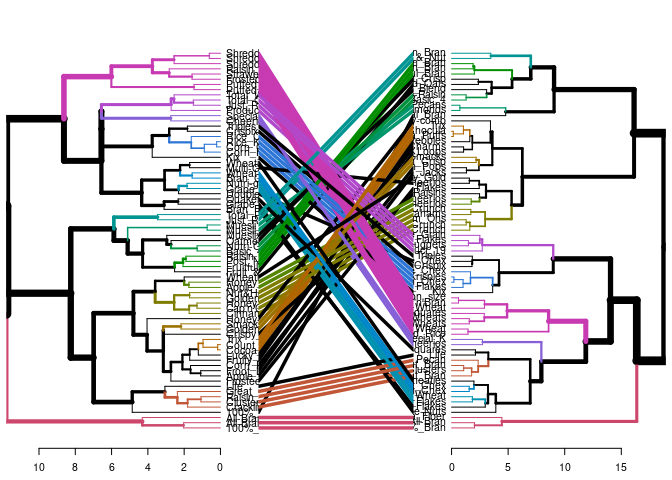
One last test of cluster stability is using Diversive Hierarchical Clustering and see how it compares to Agglomerative Hierarchical Clustering. Again, I am repeating the same process as above so I will only show the output.
DIANA Comparison
## # A tibble: 45 x 3
##    name                      cluster diana
##    <chr>                     <fct>   <fct>
##  1 100%_Bran                 1       1
##  2 100%_Natural_Bran         2       2
##  3 All-Bran                  1       1
##  4 All-Bran_with_Extra_Fiber 1       1
##  5 Apple_Cinnamon_Cheerios   3       3
##  6 Apple_Jacks               3       3
##  7 Cap'n'Crunch              3       3
##  8 Cinnamon_Toast_Crunch     3       3
##  9 Cocoa_Puffs               3       3
## 10 Corn_Chex                 5       5
## # … with 35 more rows
Very Good Cluster Stability, Again!
Performed the diana hierarchical clustering and compared it with the agnes hierarchical clustering to see if the clusters are similar for both methods which also gives evidence that the clusters are stable. Looking above you can see 45 of the 73 or about 62% cereals were grouped the same as agnes. I believe this gives further evidence of a decent clustering stability as two different clustering algorithms formed mostly the same cluster groupings.
Clustering Stability Conclusion
I believe that I can high confidence that the clusters are stable based on the two trial partition results being very high. Also, DIANA having 62% cluster similarity, I believe gives even greater confidence due to it being a different method for hierarchical clustering but still having the majority of clusters groups the same as our original clustering from the Ward’s Method using Agnes.
Healthy Cereal Recommendations
Average Clusters for Comparison
# Putting cereals into their clusters and then finding the average of each
cluster.

cereal_norm %>%
  filter(cluster == 1) %>%
  summarise_all(mean) -> cl1_ave

cereal_norm %>%
  filter(cluster == 2) %>%
  summarise_all(mean) -> cl2_ave

cereal_norm %>%
  filter(cluster == 3) %>%
  summarise_all(mean) -> cl3_ave

cereal_norm %>%
  filter(cluster == 4) %>%
  summarise_all(mean) -> cl4_ave


cereal_norm %>%
  filter(cluster == 5) %>%
  summarise_all(mean) -> cl5_ave


cereal_norm %>%
  filter(cluster == 6) %>%
  summarise_all(mean) -> cl6_ave


cluster_mean <- as.data.frame(rbind(cl1_ave,
                                    cl2_ave,
                                    cl3_ave,
                                    cl4_ave,
                                    cl5_ave,
                                    cl6_ave))

cluster_mean %>%
  relocate(shelf_1, shelf_2, shelf_3, sugars, fiber, potass) -> cluster_mean
cluster_mean <- cluster_mean[ ,c(-7, -8, -18)]

# Using "reshape2" package to rotate the average cluster dataset to
three columns "name", "variable", and "value".

library(reshape2)
cluster_mean <- melt(cluster_mean)
cluster_mean$cluster <- c(1,2,3,4,5,6)


# Healthy sugar level variable.
cereal %>%
  mutate(sugar_lvl = serving_size/4*.25) -> cereal

cereal$healthy_sugar_lvl <- ifelse(cereal$sugars <= cereal$sugar_lvl,
                                                    yes = 1,
                                                    no = 0)

# Healthy fiber levels variable.
cereal$healthy_fiber_lvl <- ifelse(cereal$fiber >= 3,
                                                   yes = 1,
                                                   no = 0)

# Healthy and high sodium levels variable.
cereal$healthy_sodium_lvl <- ifelse(cereal$sodium/cereal$serving_size <= .05,
                                                                          yes = 1,
                                                                          no = 0)

cereal$high_sodium_lvl <- ifelse(cereal$sodium/cereal$serving_size >= .2,
                                                                      yes = 1,
                                                                      no = 0)
Cluster Comparisons
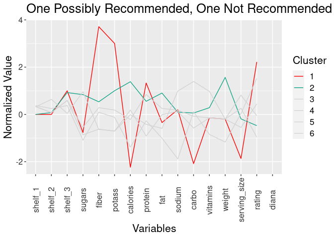
- Cluster 1: Could be Recommended
Cereals
- located on shelf 3
+ Attributes:- lower sugar
- highest fiber
- lowest calories
- lowest carbs
- highest protein
- highest rating
- Cluster 2: Not Recommended Cereals
- located on shelf 3
+ Attributes:- higher calories
- lower rating
## # A tibble: 3 x 5
##   name                cluster healthy_sugar_lvl healthy_fiber_l… high_sodium_lvl
##   <chr>               <fct>               <dbl>            <dbl>           <dbl>
## 1 100%_Bran           1                       0                1               1
## 2 All-Bran            1                       0                1               1
## 3 All-Bran_with_Extr… 1                       1                1               1
All of cluster 1 cereals all have high sodium levels. Could be on the recommendation list due to the other benefits like protein and fiber. However, kids probably would not typically choose these cereals.
## # A tibble: 13 x 5
##    name                cluster healthy_sugar_l… healthy_fiber_l… high_sodium_lvl
##    <chr>               <fct>              <dbl>            <dbl>           <dbl>
##  1 100%_Natural_Bran   2                      1                0               0
##  2 Basic_4             2                      1                0               1
##  3 Fruit_&_Fibre_Date… 2                      0                1               1
##  4 Fruitful_Bran       2                      0                1               1
##  5 Just_Right_Fruit_&… 2                      1                0               1
##  6 Muesli_Raisins,_Da… 2                      1                1               1
##  7 Muesli_Raisins,_Pe… 2                      1                1               1
##  8 Mueslix_Crispy_Ble… 2                      0                1               1
##  9 Nutri-Grain_Almond… 2                      1                1               1
## 10 Oatmeal_Raisin_Cri… 2                      0                0               1
## 11 Post_Nat._Raisin_B… 2                      0                1               1
## 12 Raisin_Bran         2                      0                1               1
## 13 Total_Raisin_Bran   2                      0                1               1
All except one cereal of cluster 2 cereals have high sodium and 7 out of 13 cereals have high sugar levels. Only 9 of the cereals have good fiber as well.

- Cluster 3: Not Recommended
Cereals
- located on shelves 1 & 2
+ Attributes:- highest sugar
- low fiber
- lowest protein
- lower carbs
- lowest rating
- located on shelves 1 & 2
- Cluster 4: Not Recommended
Cereal
- located on shelves 1 & 3
+ Attributes:- lower sugar
- lowest fiber
- higher protein
- higher rating
- located on shelves 1 & 3
cereal %>%
  filter(cluster == 3) %>%
  select(name, cluster,  healthy_sugar_lvl, healthy_fiber_lvl, high_sodium_lvl)

## # A tibble: 22 x 5
##    name               cluster healthy_sugar_lvl healthy_fiber_l… high_sodium_lvl
##    <chr>              <fct>               <dbl>            <dbl>           <dbl>
##  1 Apple_Cinnamon_Ch… 3                       0                0               1
##  2 Apple_Jacks        3                       0                0               1
##  3 Cap'n'Crunch       3                       0                0               1
##  4 Cinnamon_Toast_Cr… 3                       1                0               1
##  5 Cocoa_Puffs        3                       0                0               1
##  6 Corn_Pops          3                       1                0               1
##  7 Count_Chocula      3                       0                0               1
##  8 Crispy_Wheat_&_Ra… 3                       0                0               1
##  9 Froot_Loops        3                       0                0               1
## 10 Frosted_Flakes     3                       0                0               1
## # … with 12 more rows
13 of the cereals in cluster 3 have unhealthy sugar levels and none of them have healthy fiber or sodium levels. Kids should not consume these.
cereal %>%
  filter(cluster == 4) %>%
  select(name, cluster, healthy_sugar_lvl, healthy_fiber_lvl, high_sodium_lvl)

## # A tibble: 15 x 5
##    name               cluster healthy_sugar_lvl healthy_fiber_l… high_sodium_lvl
##    <chr>              <fct>               <dbl>            <dbl>           <dbl>
##  1 Bran_Chex          4                       1                1               1
##  2 Bran_Flakes        4                       1                1               1
##  3 Cheerios           4                       1                0               1
##  4 Clusters           4                       0                0               1
##  5 Cracklin'_Oat_Bran 4                       0                1               1
##  6 Grape_Nuts_Flakes  4                       1                1               1
##  7 Grape-Nuts         4                       1                1               1
##  8 Great_Grains_Pecan 4                       1                1               1
##  9 Life               4                       1                0               1
## 10 Nutri-grain_Wheat  4                       1                1               1
## 11 Quaker_Oat_Squares 4                       1                0               1
## 12 Raisin_Nut_Bran    4                       0                0               1
## 13 Special_K          4                       1                0               1
## 14 Wheat_Chex         4                       1                1               1
## 15 Wheaties           4                       1                1               1
13 of the cereals in cluster 4 have healthy sugar levels. 14 cereals do not have healthy fiber levels and they all have high sodium. The only factor that cluster 3 has going for it is the sugar levels but I don’t believe that is enough to recommend it as the other “unhealthy” factors outweigh that benefit.
- Cluster 5: Not Recommended
Cereals
- located on shelves 1 & 3
+ Attributes:- lower sugars
- lower fiber
- high sodium
- high carbs
- high vitamins
- located on shelves 1 & 3
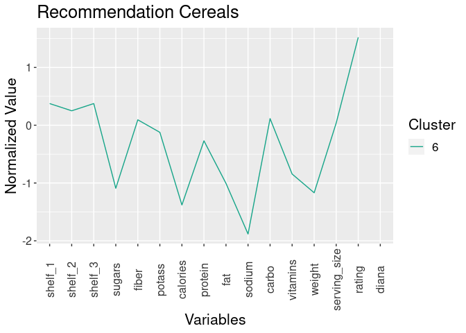
- Cluster 6: Recommended
Cereals
- located on shelves 1 & 3
+ Attributes:- loweest sugar
- lower calories
- lowest sodium
- high rating
- located on shelves 1 & 3
cereal %>%
  filter(cluster == 5) %>%
  select(name, cluster, healthy_sugar_lvl, healthy_fiber_lvl, high_sodium_lvl)

## # A tibble: 12 x 5
##    name               cluster healthy_sugar_lvl healthy_fiber_l… high_sodium_lvl
##    <chr>              <fct>               <dbl>            <dbl>           <dbl>
##  1 Corn_Chex          5                       1                0               1
##  2 Corn_Flakes        5                       1                0               1
##  3 Crispix            5                       1                0               1
##  4 Double_Chex        5                       1                0               1
##  5 Just_Right_Crunch… 5                       1                0               1
##  6 Kix                5                       1                0               1
##  7 Product_19         5                       1                0               1
##  8 Rice_Chex          5                       1                0               1
##  9 Rice_Krispies      5                       1                0               1
## 10 Total_Corn_Flakes  5                       1                0               1
## 11 Total_Whole_Grain  5                       1                1               1
## 12 Triples            5                       1                0               1
All of cluster 5 cereals have healthy sugar levels but have high sodium and all but one do not have enough fiber. Although they do have high vitamins which could be a benefit but hard to determine from this dataset. Overall I don’t believe that the healthy sugar levels and high vitamins are enough to recommend as the sodium levels are the highest and the fiber is lower compared to the other clusters.
cereal %>%
  filter(cluster == 6) %>%
  select(name, cluster, healthy_sugar_lvl, healthy_sodium_lvl, healthy_fiber_lvl)

## # A tibble: 8 x 5
##   name              cluster healthy_sugar_lvl healthy_sodium_l… healthy_fiber_l…
##   <chr>             <fct>               <dbl>             <dbl>            <dbl>
## 1 Frosted_Mini-Whe… 6                       1                 1                1
## 2 Puffed_Rice       6                       1                 1                0
## 3 Puffed_Wheat      6                       1                 1                0
## 4 Raisin_Squares    6                       1                 1                0
## 5 Shredded_Wheat    6                       1                 1                1
## 6 Shredded_Wheat_'… 6                       1                 1                1
## 7 Shredded_Wheat_s… 6                       1                 1                1
## 8 Strawberry_Fruit… 6                       1                 0                1
All of cluster 6 cereals have healthy sugar levels, 7 of the cereals have healthy sodium levels, and 5 have healthy fiber levels. Overall, these are cereals are better for kids than the other cereals. Kids also would eat these cereals. It also has a variety of cereals for kids to choose from and some of them are surprising like frosted mini-wheats…who would have guessed?!
Cereal Recommendation
I recommend cluster 6 cereals* for my children based on the reasons
listed above. However, if my kids refused those cereals then Cluster 4
would be my second recommendation due to the amount of cereals with
healthy sugar and fiber levels. Although their blood pressure might
suffer due to the sodium…parenting is not easy…